Application of MLE
Choosing the values that make the observed data most likely is key to the MLE method. It does not minimize errors, like in traditional regression, but centers around probability, and converts the variables into parameters that best describe the real-world outcomes and chances that are logged. This helps predict, using the data inputs, models for financial institutions or companies to use as a point of reference for their decision making.
This is especially important in econometric modeling, as many economic and financial variables cannot be simplified as continuous numbers. They can involve binary outcomes such as yes/no conditions, or pivot on censored data or even grouped information, which standard linear regression does not accurately factor in.
Applying MLE to Incomplete and Non-Linear Datasets
The practicalities of MLE are most clear when in direct comparison with traditional regression techniques. Where these techniques focus on minimizing errors and extrapolating linear outcomes, Maximum Likelihood Estimation makes the most of these errors. It converts these raw variables into parameters that provide a more holistic and less rounded or biased model to explain the real-world outcomes.
In economic data and financial research there are rarely any real world applications that are simple or completely continuous. In scenarios where there are binary outcomes with yes/no answers, censored data where values are only partially observed, or grouped data that only shows outcomes within a defined range, there are variables that are not fully complete, nor compatible with each other.
Real World Data Inputs
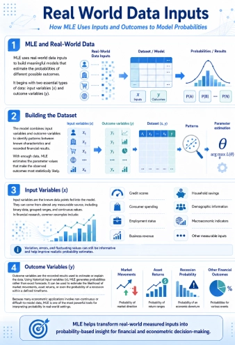
MLE provides a way for these data inputs to be plugged into complex datasets and provide meaningful models to determine the probabilities of different possible outcomes. This all starts with the inputs themselves. MLE requires two types of data, the input variables (x) and the outcome variables (y).
The model needs the input variables and outcome variables to create datasets, which can then be used to identify patterns between known characteristics and recorded financial results. When enough data is collected, highly precise models can be generated, estimating the parameter values that make the outcomes most statistically likely.
Input Variables
The input variables are the known data points that are fed into the model. These can come from virtually any source that can be measured, no matter whether it is a binary yes/no input or a grouped range of data. Typically, in financial research the input data can relate to:
- Credit scores
- Consumer spending
- Employment status
- Business revenue
- Household savings
- Demographic information
- Macroeconomic indicators
And anything that is measurable through any of the data input methods. The idea is to maximize probability here, so errors, variance or fluctuating values are all useful as they can generate a more accurate outcome.
Outcome Variables
The common outcome variables (y) are the recorded results from the calculations, which project the inputs to make estimations or explain the data. There are many applications for MLE outcomes, and with scalable formulae and flexible result generation, it can be tweaked with more variables or inputs.
Essentially, these use the historical data, or input variables (x), to generate probabilities. It can be used to predict the direction of a market movement, the size of an asset return over time, or even more vague examples like the probability of a recession occuring in a strict timeframe. As such, the data must be carefully handled and aggregated to achieve the most accurate results. Rather than giving precise forecasts, the system analyzes the likelihood of different possible outcomes. As many econometric applications do not have continuous values or directly compatible data inputs, MLE is one of the most powerful tools to accurately interpret probability in real world applications.
Different Outcomes in MLE Models
Maximum Likelihood Estimation can manage a diverse range of data inputs, which is one of its great strengths for data and financial analysts. So long as a piece of data is measurable, it can be applied into the model without needing tweaks, alternative interpretations, or conversion into an alternate expression, which is where errors or rounding can taint the results. The ability to handle multiple types of outcomes, incomplete or even limited datasets is what makes MLE an optimal tool for financial research.
Choosing the MLE system revolves around the structure of the data input itself. For instance, there are models that focus on binary outcomes, where yes/no data inputs are analyzed. Others may focus on continuous numerical values, or even partial data sets. Each structure requires a different probability distribution and estimation method, through which they can reflect the real world conditions driving the data and accurately examine the errors, and generate the future outcome probabilities.
Binary Outcomes
Binary outcomes are the most common in MLE models, and they can relate to a plethora of different measurable data. It is anything that is limited to just two possible results, which can b yes/no, approve/reject, buy/not buy, or rise/fall, depending on what scenario is being measured. The MLE is superior to the standard linear regression systems simply because those methods are not suited to scenarios that remain between 0 and 1, or yes/no.
In practise, MLE solve the binary outcomes using probability-based systems, like the Logit or Probit models. These can use the input data to project estimated probabilities on the outcomes, in the form of a probability score. It is highly effective for any risk analysis, market projections, and other financial research that has many 2-result data inputs and needs a percentage or probability scoring to give the user an idea of what to expect.
Continuous Values
Continuous values relate to outcome variables that span a bigger range of numerical values. These can be inflation rates, asset prices, GDP growth figures, or any other data inputs that have a range of values, which are connected in time or to a singular property. The idea is that the MLE can plug these values, without overlooking errors or discrepancies but in fact using these to generate a probability distribution.
This method is one of the de facto systems used in quantitative finance and macroeconomic forecasting. These are areas where inputs can have wildly fluctuating numerical values, unknown external variables to create discrepancies or larger jumps, and the MLE method maximizes these. It will not create a distribution based on the most frequent or seemingly significant data, but take all the larger deviations and isolated data inputs, and generate probability distributions to factor these in. It is not only used to project future probabilities, but MLE can also be used to explain or find answers for historical data discrepancies.
Censored Data
Any data that is incomplete or notably limited by a threshold is classified as censored data. These are the inputs where analysts do not have precise results, because they fall above or below a certain level, or where the reports are not fully complete. Instead of discarding this information, in MLE it can be applied in systems like the Tobit method.
The linear regression systems, used in traditional financial research, cannot cover these gaps because the missing information can distort the final outcome. Instead, they are either converted or rounded into variables that can be applied, or they are, where possibly, omitted from the models to avoid tainted results. MLE on the other hand has censored data based models, such as Tobit, which can solve the incomplete datasets by plugging the partial data into the estimation process. It does not get ignored, minimized, or rounded to create biased results.
Grouped Information
Grouped information is similar to censored data, as these have limits, but the limits are prescribed to specific ranges or categories. In many cases, these numbers may be ranges or not exact figures. Other cases may just include data for exclusive categories or scenarios. For instance, data from demographic studies, income ranges, spending categories, or types of group investment data.
Instead of opening these ranges or converting them to meet an all encompassing formula, MLE can generate accurate estimates by calculating within those grouped data ranges. The model does not require exact values for each data point, it works within the grouped interval, and maximizes the probabilities. It is highly useful for scenarios where datasets are partially complete or restricted to specific ranges, and traditional systems cannot properly discern the data without making broad assumptions.
MLE in Econometric Modeling
After going through the different types of input datasets, now we can apply them into the various MLE models. These have to be generated in different probability models, depending on the coefficients or the datasets. Then, they can be joined into one expression to calculate different likelihoods, explain discrepancies, and convert complex values into simpler ones. Each different system provides its own outcome, and for some types of data inputs, there are several models that can be used, each to meet a slightly different end.
For using MLE is not just a case of plugging data for simpler outcomes. Choosing the system very much hangs on the final outcome that analysts are after. Whether they want to create interpretable odds ratios, which Logit is ideal for, or find normally distributed error terms, where the Probit is more effective.
Logit Systems
- Input: Binary
- Formula: Uses logistic probability distribution
- Outcome: Probability score between 0 and 1
One of the most commonly used MLE models, Logit requires binary inputs. These are converted into probability scores that remain between 0 and 1, by applying a logistic distribution from the input variables. Logit is used to estimate probability for a certain outcome to occur, in easily understandable terms.
The results can show researchers which variables have the strongest impacts on the outcomes, which is good for finding errors or distinguishing frequently occuring data patterns. It also determines how sensitive the outcomes are to these changing inputs.
Probit Models
- Input: Binary
- Formula: Cumulative normal distribution functions
- Outcome: Probability score between 0 and 1
Probit is similar to Logit, but the difference is that instead of using a logistic distribution it uses a standard normal distribution model. This means Probit can transform linear data inputs into a probability score, and has stronger results for outcomes that follow normal latent structures. It is a more assumptive approach, which is useful for making financial decisions, such as deciding whether to approve a credit request, or whether or not an investment with binary outcomes is worth risking or not.
This method works best without extreme outcomes, as the normal distribution does not distort as much in these scenarios. Where there are more extremes, Logit is prefreable. Probit is generally used for more conservative risk modeling assessment, but it has its limits.
Tobit Systems
- Input: Censored data or grouped
- Formula: MLE with censored limits
- Outcome: Continuous latent variable
Tobit systems can maximize the likelihood estimations in limited ranges of data. Where there are censored data inputs, and thus the results are either limited within strict thresholds or they are partially incomplete, Tobit can create latent variables along a normal distribution. That means, creating a hidden variable that cannot be directly measured, but it can be inferred from other variables that are measured.
The Tobit system evaluates the value of the distribution within these ranges, but it can also predict the probability of the data getting censored, which is useful for historical analysis.
Interval Regression Systems
- Input: Interval censored data and grouped inputs
- Formula: MLE over bounded intervals, not exact points
- Outcome: Latent variable within given ranges
Interval regression systems can maximize probabilities where the data inputs are incomplete or the exact numbers are not given. The key is to note the intervals, and the model can find parameters that maximize probabilities from these partial or grouped datasets.
For instance, when the data input is not 1, but an interval of 1-5, then the interval regression system can estimate a latent variable continuing from this variable into the next. It accommodates any lost or partial datasets so that they can be used to improve the overall model accuracy. Without interval regression systems, these datasets would get excluded, or rounded, creating a form of measurement bias or censorship.
Examples of MLE in Real World Economics
Maximum Likelihood Estimation is the ideal tool for handling financial data that comes with different inputs. It does not matter if the information is limited, not an exact figure, spans a larger range of values, or is limited to just 0 and 1. For instance, it can be used in banking to calculate a loan default prediction. Based on varying datasets such as credit scores, customer income, and whether or not there were defaults in previous credit loans, the banks can maximize the likelihood of a default, and use it to explain discrepancies or blips in a person's default history.
MLE can also be used to generate asset return modeling. It does not skip on any datasets or information, encompassing macroeconomic variables, inflation data, spending and market volume to create a distribution of the observed price returns. Risk analysis and explaining extreme price movements can be done within the same formula, maximizing the use of these mathematical systems.